An uncalibrated model, checked against a real gauge
Automatic model building is easy to claim and hard to prove. So SWMMCanada is measured three ways: against an independent flow gauge, against the EPA SWMM engine itself, and against the cities' own published network data.
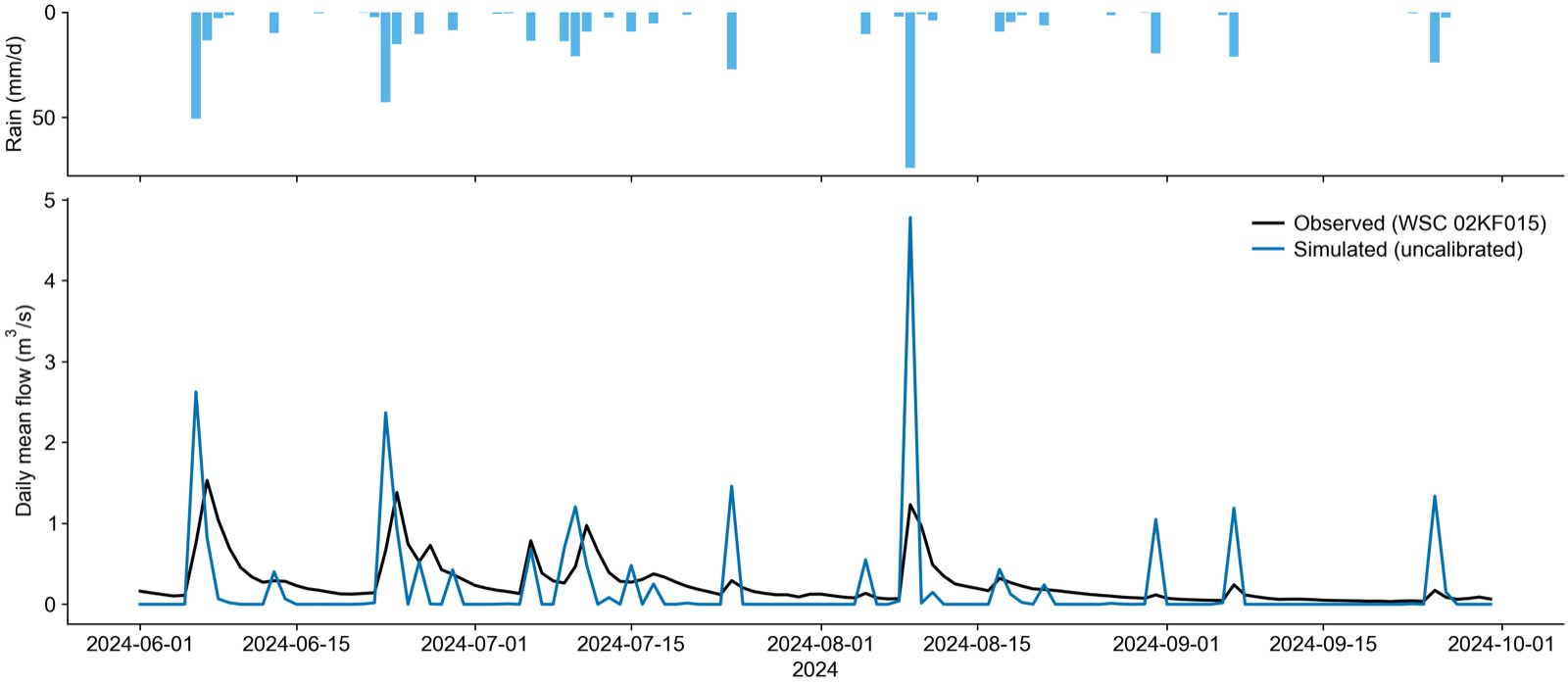
All 12 rainfall events, on the correct days
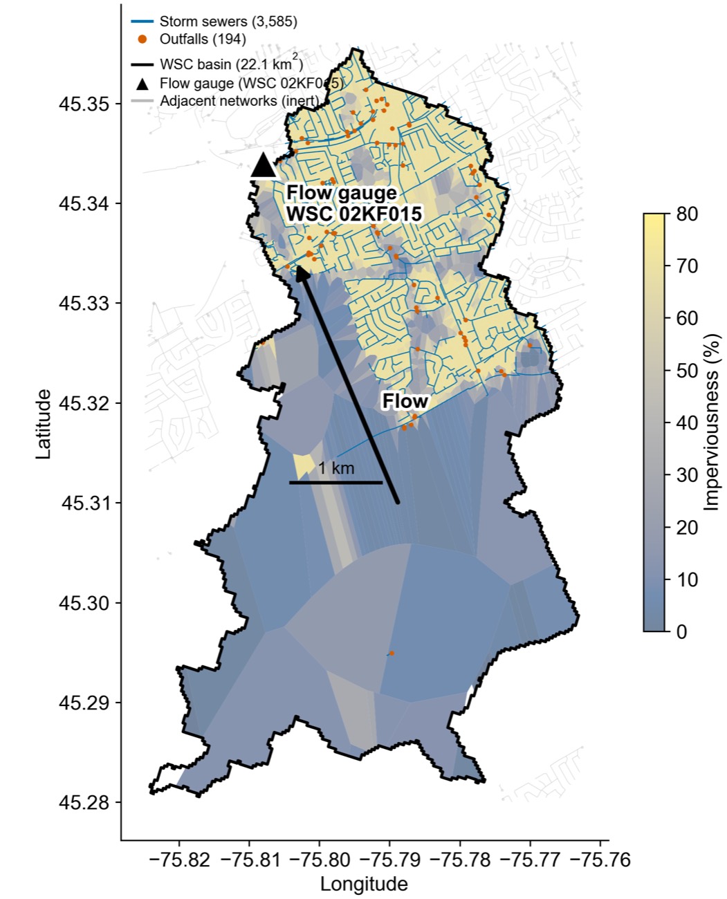
One question: if SWMMCanada builds a model with zero manual input and zero calibration, how close does it get to a real flow gauge? The test basin is Graham Creek at Nepean, Water Survey of Canada station 02KF015 — a 22.09 km² gauged basin in Ottawa. The area of interest is the official WSC drainage polygon, not a hand-drawn box, so the model drains exactly what the gauge measures.
Why this basin is a hard test
Graham Creek is half and half. The northern half is suburban Bells Corners — 60–80% impervious, densely sewered (3,585 municipal conduits, 3,550 manholes and 194 outfalls straight from Ottawa's open data). The southern half is National Capital Commission greenbelt including the Stony Swamp wetlands: imperviousness near zero, no sewers at all. A mixed urban–greenbelt basin is harder than a fully urban one, because the model has to get both the fast city water and the slow greenbelt water right.
The numbers, read honestly
| Metric | Value | What it means |
|---|---|---|
| Event detection | 12 / 12, same day | The rainfall → runoff → network → outflow chain is causally right. |
| Volume bias (PBIAS) | −22.3% | The correct order of magnitude with no tuning and no baseflow. |
| Wet-day mean (34 d) | sim 0.696 vs obs 0.473 m³/s (+47%) | A sewer-network model has no in-stream or wetland storage; the real creek crosses the Stony Swamp wetlands, which attenuate every peak. |
| Dry-day mean (88 d) | sim 0.001 vs obs 0.165 m³/s | The gap is groundwater baseflow — which a storm-runoff model deliberately does not simulate. |
| Daily NSE | −2.49 | Dominated by the two structural gaps above, not by random error. |
| Monthly means (sim / obs) | Jun 0.28/0.42 · Jul 0.17/0.29 · Aug 0.24/0.22 · Sep 0.09/0.07 | August and September nearly coincide. |
The engine's own mass balance for the 122-day run: runoff continuity −0.16%, routing continuity −0.98%, both well inside SWMM's ±2% guideline. Of 448.5 mm of rain, 311 mm infiltrated (the greenbelt half at work), 23 mm evaporated, and 115 mm became runoff.
The error is explainable, not random. Two structural gaps account for it: no baseflow on dry days, and no wetland or in-stream storage on wet days. Both are consequences of modelling a pipe network rather than a creek — and both are stated rather than tuned away.
Every model is run, not just written
A model that assembles but will not execute is worth nothing, so real-city builds are run in the EPA SWMM 5.2 engine as part of validation — checked for zero engine errors and for mass-balance continuity inside SWMM's ±2% guideline. The Graham Creek run above closed at −0.16% runoff and −0.98% routing continuity over 122 days.
"Zero engine errors" means runnable, not calibrated. Every result on this page confirms that the model is structurally sound and executes without error. It is not a claim that the hydrology is accurate — parameters are first-pass estimates from open data. Calibrate against observations before using any output for design or decisions.
The generated network is the city's network
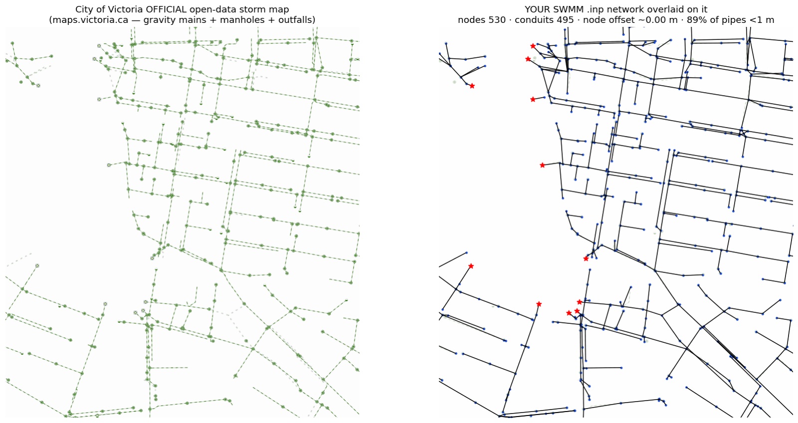
Victoria publishes storm mains with explicit topology, invert elevations, diameters and materials, so the built network can be checked field by field against the city's own map. Node positions are an exact copy of the source manholes and outfalls (0 m offset), and 89% of conduits lie within 1 m of the real pipe centreline (95% within 5 m) — the small residual is the straight node-to-node representation of a curved polyline.
Where a city publishes no node IDs
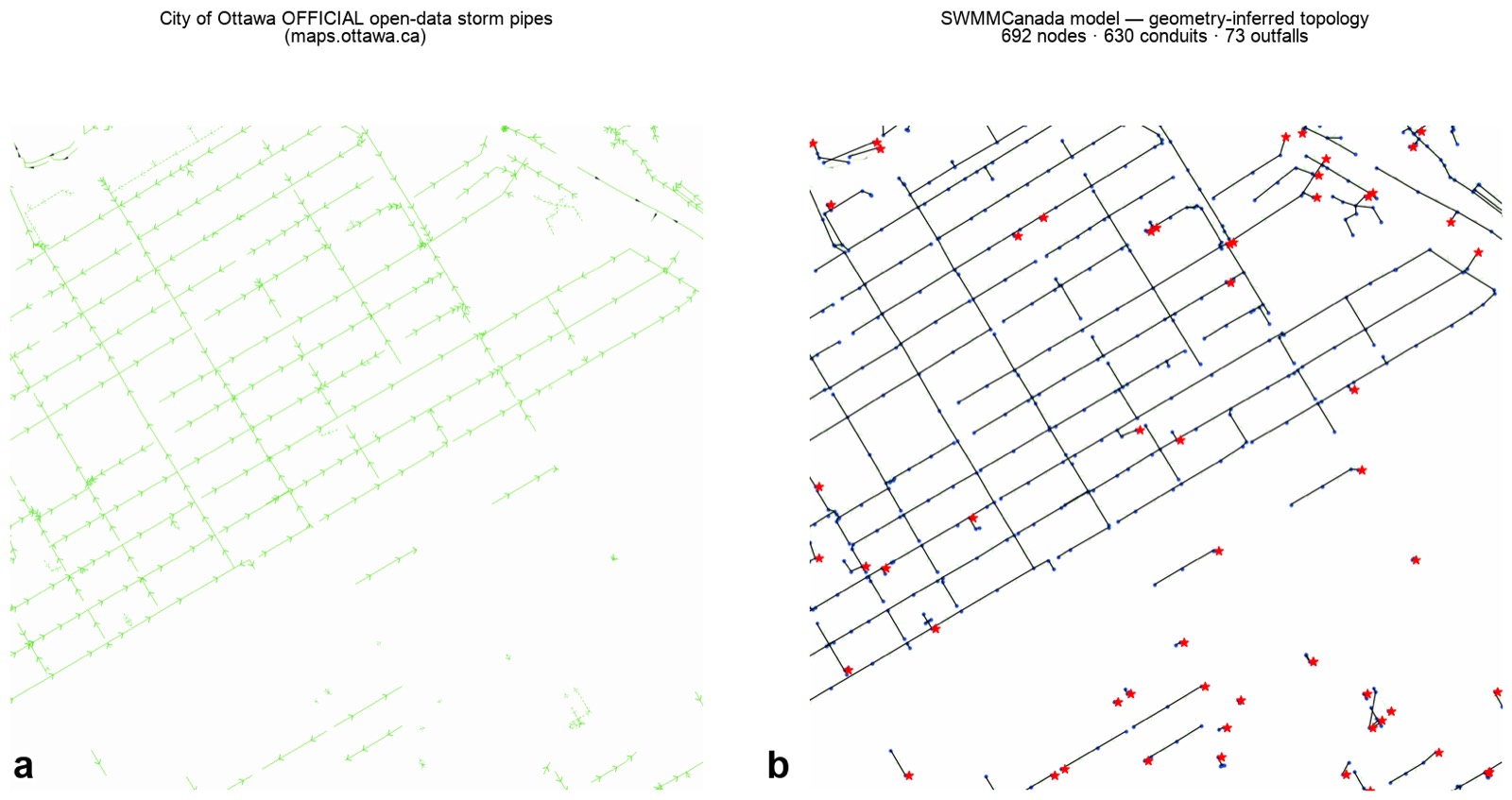
Ottawa publishes inverts, diameters and materials but no node IDs, so the topology is reconstructed by snapping pipe endpoints to shared nodes — the same shared assembler handles both cases. Outfalls come from the city's outlet layer plus a sink per disconnected component, so the network is always mass-balanced.
Subcatchments on real lot lines
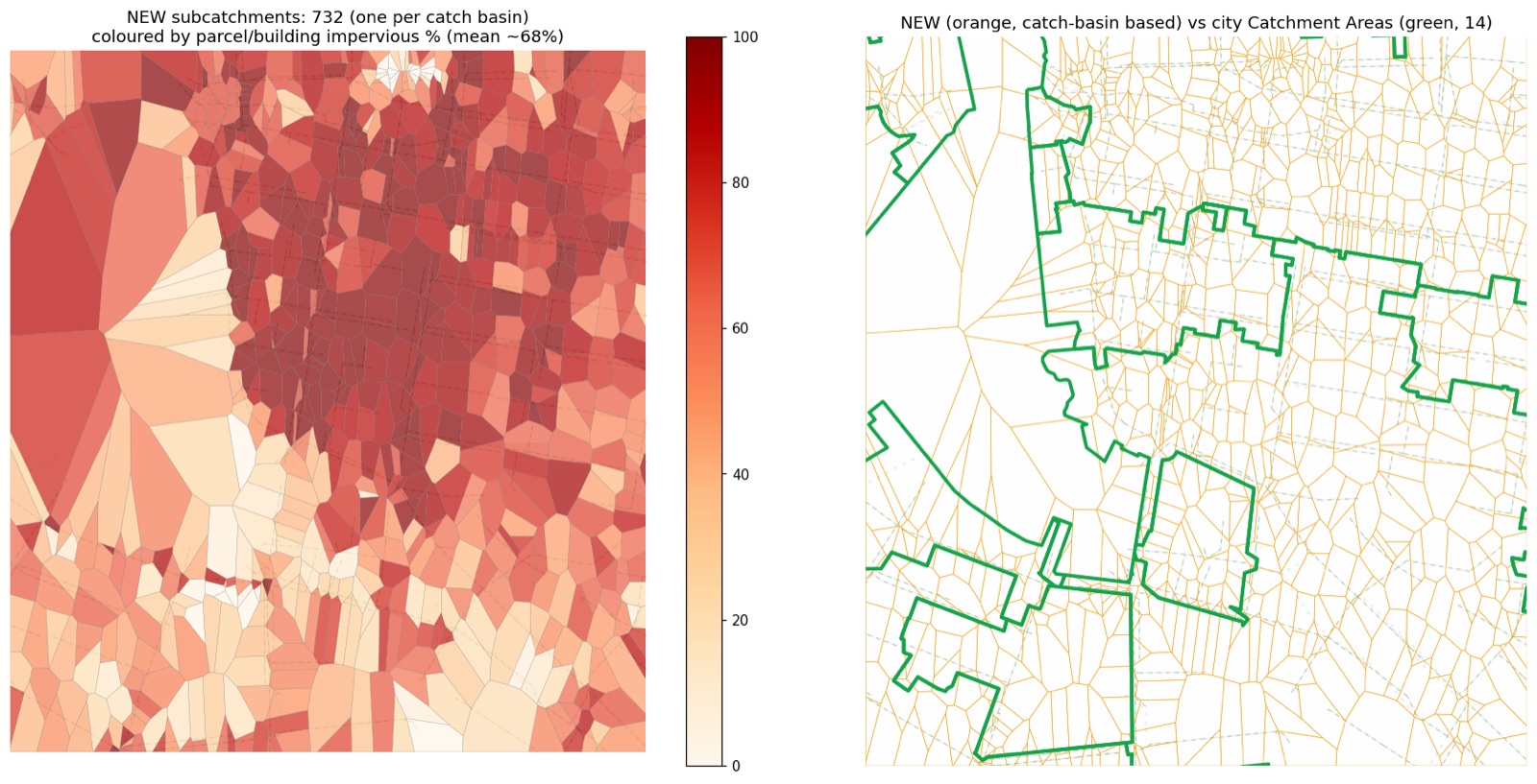
Where a city publishes parcels and building footprints, drainage units are seeded on the real catch basins and shaped by real lot lines, with imperviousness from real buildings plus road right-of-way — far finer than a 30 m land-cover raster.
DEM catchments — but only where the terrain earns it
Subcatchments can be delineated from the conditioned DEM: depressions filled, OpenStreetMap streets burned in so urban flow follows roads, and D8 basins traced to each manhole. On flat ground that is false precision — a 30 m national DEM with ±1–2 m accuracy cannot resolve which side of a downtown street a raindrop runs down. So a two-layer honesty gate decides per area and records its readings in the validation report, with a resolution-aware threshold:
- Below 4.0% median conditioned slope at ≥10 m DEM posting, the delineation honestly stays geometric (junction-Voronoi).
- Under LiDAR (≤2 m posting, ~0.1–0.2 m accuracy) the threshold drops to 1.0% — at that resolution urban micro-slope is real signal, not noise.
- A DEM result that fails validation falls back automatically.
The 4.0% default is measured, not guessed: seven downtown areas read 1.1–3.3% median slope (inside DEM noise → Voronoi), while a Kelowna hillside reads 9.12% and North Vancouver slopes read 13.25% (→ DEM basins). Downtown Ottawa, resolved onto the city's own 2020 LiDAR at 1 m, reads 2.52% — above the fine gate — and upgrades to 442 DEM basins with zero errors and 0.0% uncovered area, in 42 seconds.
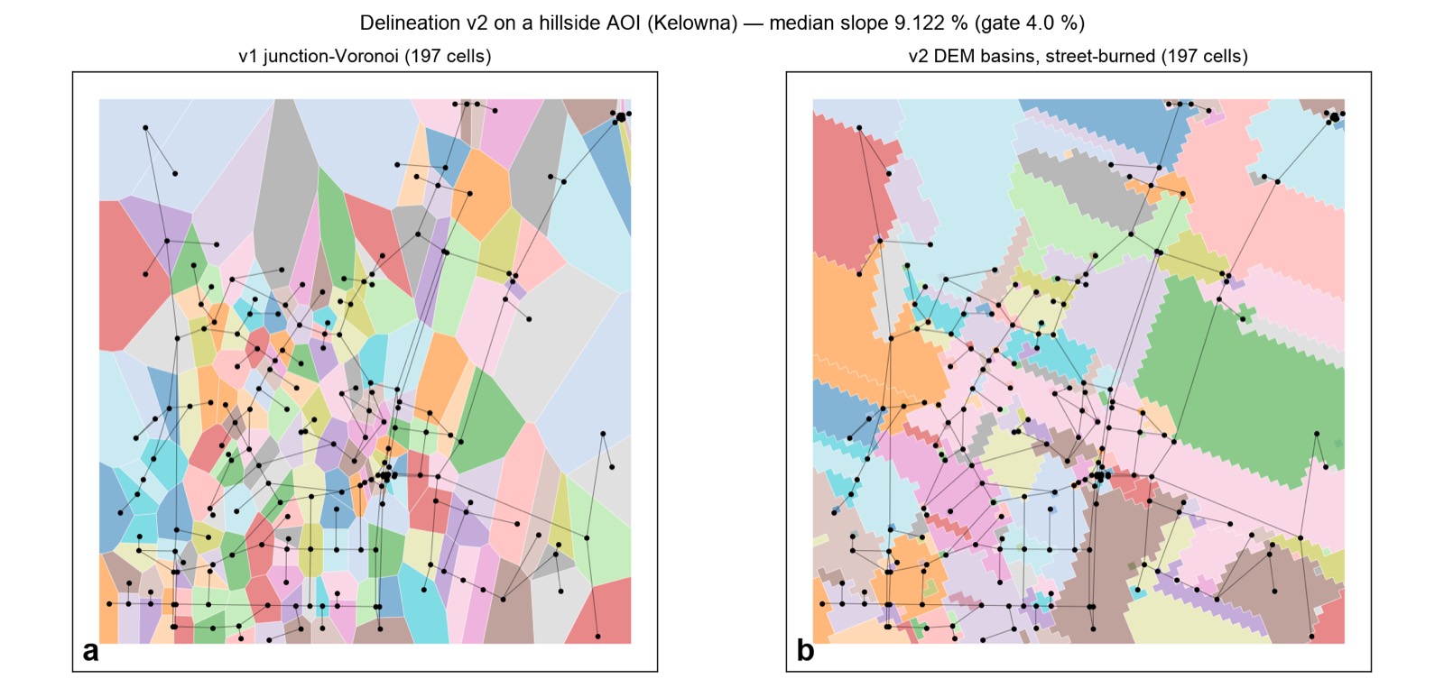
Regression baselines lock today's delineation verdict on checked-in fixtures, so a future change to the method has to move them in a reviewed diff — it cannot silently degrade coverage.
Go deeper
RESULTS.md →
The full validation write-up: engine numbers, the delineation gate, and the reproduction scripts.
Graham Creek →
The gauge case study in full, including how to reproduce it from HYDAT.
Data tiers →
How complete each city's vertical data really is — A, B, or C, with the measured typical error.
ASSUMPTIONS.md →
What's real, derived, or approximated in a model, layer by layer.